|
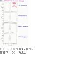
The most annoying and irreducible example of the consequences
of this defective model is the ``ringing'' due to
different frequencies matching or mismatching the endpoint
of a finite time spectrum. To combat this effect, one can use
the technique of apodization, in which the time spectrum
is multiplied by an ``envelope'' function (a sort of artifical
relaxation function) which smoothly reduces the oscillatory signal
to zero at the end of the time range. This artificially broadens
the resulting frequency spectrum, of course,
[From David Spencer's Ph.D. thesis, ~ 1980] |
|
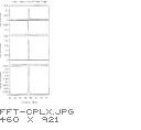
Apodization is especially needed when, through a flaw in the
counting electronics or just sheer bad luck in counting statistics,
one time bin has an anomalously high or low value.
[From Tanya Riseman's Ph.D. thesis, 1993] |
|
In this case the frequency spectrum will exhibit a huge oscillation
over its entire range (think what a single ``spike'' in a frequency
spectrum means about the time spectrum, and then reason backwards).
[From Tanya Riseman's Ph.D. thesis, 1993] |
|
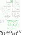
Another aspect of the FFT that is often overlooked is the fact that its output is a mixture of a real part that can be quite sharp since it is the cosine function (which is an even function and therefore doesn't mind starting abruptly at t=0) and an imaginary (sine function) part which does mind, and which has an enormous extra broadening because it is the transform of the Heaviside function. If the two are simply added in quadrature (or squared to produce the power spectrum) this superfluous broadening wipes out any fine structure in the frequency spectrum. At high fields it is no simple matter to separate the real and imaginary parts; this can be done numerically, but only to limited precision, leaving a spectrum with unknown (and probably unknowable) distortions. |
|
Many other problems are encountered by the determined Fourier transformer seeking an aesthetically pleasing frequency spectrum; most of these can be overcome sufficiently to satisfy the observer, as illustrated here, but one should never forget that all model-independent transformations from the time domain into the frequency domain involve arbitrary and fundamentally unreliable quantitative decisions by the transformer, and should therefore be regarded as qualitative illustrations, never as reliable quantitative measurements. |
|
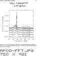
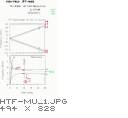
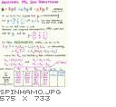
Actually the first (and most unambiguously useful) applications of FT-µSR were to complex spin systems in which the muon polarization oscillates at many frequencies simultaneously. Of the many examples available, I chose the classic study of Mu* in semiconductors as an illustration. Whereas ESR (or EPR if you prefer) usually probes the spin Hamiltonian by sweeping the magnetic field through the resonances on the Breit-Rabi diagram at fixed RF frequency, FT-µSR reveals all the frequencies at once for a given magnetic field. |
|
In gallium arsenide (like many other semiconductors, fortuitously excluding Si, Ge and diamond) the nuclei have their own HF interaction with the muonium electron, broadening the lines so dramatically at low field that they cannot be observed in TF-µSR. Fortunately, at high field (in this case 1.2 T) the nuclear hyperfine (NHF) splittings are reduced to the point where the muonium HF structure can be seen clearly. |
|
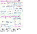
These formulae show how the muon polarization evolves in strong transverse field (TF) and longitudinal field (LF) assuming (often incorrectly) a scalar (isotropic) Mu HF interaction. |
|
In most semiconductors and insulators muonium experiences an anisotropic spin hamiltonian. |
|
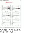
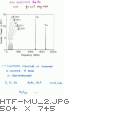
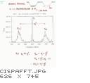
Another important use of FT-µSR is in the spectroscopy of radicals. Rather than show one of the many examples from muonium chemistry, I have chosen the rather exotic case of cis-polyacetylene, a solid composed of the cis isomer of polyacetylene (the trans isomer forms an organic semiconductor). Notice the partially resolved NHF structure in the solid; in liquids, these splittings tend to be averaged away by rapid rotation and tumbling of the molecules. |