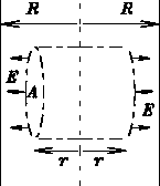
- (a)
- Using only (i) the SUPERPOSITION PRINCIPLE for the total electric field due to an assembly of electric charges, plus (ii) simple SYMMETRY arguments, deduce the direction of the electric field due to the plane of charge.
- (b)
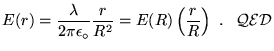
- Using the preceding result plus the general ideas of GAUSS' LAW and simple geometry, deduce the dependence of the magnitude E of the electric field upon x, the perpendicular distance away from the plane.
- (c)
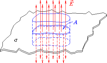
- Show that your result agrees with the x-dependence of
the electric field on axis due to a uniform disc of charge
when
 ,
the radius of the disc.
,
the radius of the disc.
![$\ds{ E(x) = {\sigma \over 2 \epsilon_0}
\left[ 1 - {x \over \sqrt{ x^2 + R^2 }} \right] }$](img8.gif) for a disc. For
for a disc. For
ANSWER:
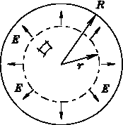
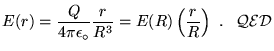
By Gauss' Law,
![]() where
where
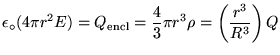
![]() is the total charge inside the closed Gaussian surface:
if we use a sphere of radius r<R then
is the total charge inside the closed Gaussian surface:
if we use a sphere of radius r<R then
![]() .
By spherical symmetry,
.
By spherical symmetry, ![]() points radially outward
(normal to the surface) and is the same strength all over the sphere,
so Gauss' Law yields
points radially outward
(normal to the surface) and is the same strength all over the sphere,
so Gauss' Law yields
![]() , giving
, giving
![\fbox{ $\ds{ E = \left( Ze \over 4\pi\varepsilon_0 \right)
\left( 1 \over R^2 \right)
\left[ {R^2 \over r^2} - {r \over R} \right] }$\space for $r<R$\space }](img19.gif) .
.
At r=R this goes to zero; for r>R
there are equal amounts of positive and negative charge
enclosed, so Gauss' Law tells us that
![]() .
Now to calculate the potential
.
Now to calculate the potential ![]() :
:
If we take the potential to be zero for
![]() ,
,
![]() ,
then integrating
-E(r') dr' from r'=R to r'=r
(the same thing as integrating E(r') dr' from r'=r to r'=R)
gives
,
then integrating
-E(r') dr' from r'=R to r'=r
(the same thing as integrating E(r') dr' from r'=r to r'=R)
gives
The integral can be split into two parts,
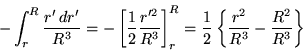
Although these are not hard integrals, one can easily fall into confusion by not thinking carefully about the limits of integration. Since R2/R3 = 1/R, we can combine the two results to give
![\fbox{ $\ds{ \phi(r<R) = \left( Ze \over 4\pi\varepsilon_0 \right)
\left( 1\ov . . .
. . . \left[
{R \over r} + {1\over2}{r^2 \over R^2} - {3\over2} \right]
}$\space }](img26.gif) .
The plots looks like this:
.
The plots looks like this:
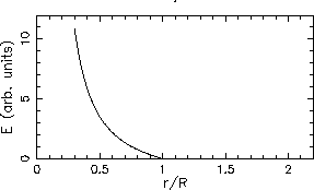
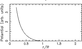
The two graphs have qualitatively similar behaviour - each ``blows up'' as
ANSWER:
Sphere:
Cylinder:
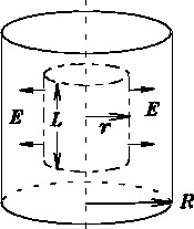
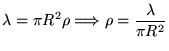
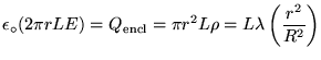
Slab: