THE UNIVERSITY OF BRITISH COLUMBIA
Physics 210
Assignment #
8:
MATRIX MADNESS!
Tue. 28 Oct. 2008 - finish by Tue. 4 Nov.
Since the course descriptions headlines MatLab,
let's do something truly "computational" with it.
As usual, create your ~/HW/08/ directory to store your work in.
- MATLAB WARMUP:
Remember the Fibonacci numbers from Assignment 7?
In a file fibmat.m,
write a MatLab function to do the same thing.
While you're at it, plot the resulting
 as a function of
  so it will be easy to check your work.
Store your plot in
so it will be easy to check your work.
Store your plot in ~/HW/08/fib.pdf
(using ImageMagick's convert if necessary).
- PAULI MATRICES:
The most important matrices in Physics (so say I)
are the Pauli spin matrices, described accurately in
the WikipediA1 as "a set of
 complex Hermitian and unitary matrices . . . "
![$\displaystyle \sigma_1 = \left[\begin{matrix}0 & 1 \cr 1 & 0 \end{matrix}\right . . .
. . . \right]; \; \sigma_3 = \left[\begin{matrix}1 & 0 \cr 0 & -1 \end{matrix}\right]$](img4.gif) |
(1) |
which can represent (among other things) the three components
(
 ,
,
 and
and
 ) of the vector spin operator
 for a spin-
 particle.2
Well, MatLab claims to be a "Matrix Laboratory",
so it should be an ideal platform for verifying the essential
properties of the Pauli matrices.3
Do so, for the list of properties listed on
particle.2
Well, MatLab claims to be a "Matrix Laboratory",
so it should be an ideal platform for verifying the essential
properties of the Pauli matrices.3
Do so, for the list of properties listed on
http://en.wikipedia.org/wiki/Pauli_matrices
down to the beginning of the subject heading labelled " ".
Make sure you understand the meaning of all these properties
thoroughly.4
".
Make sure you understand the meaning of all these properties
thoroughly.4
In this notation, the spin state of a spin-
particle
is represented by a 2-component column vector, like
![$\displaystyle \vert \! \uparrow \rangle = \left[ 1 \atop 0 \right] \qquad \hbox{\rm and} \qquad \vert \! \downarrow \rangle = \left[ 0 \atop 1 \right]$](img12.gif) |
(2) |
for "spin up" and "spin down" (along the  axis)
respectively.
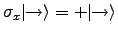
Verify that operating on these column vectors from the left
with the Pauli matrix
axis)
respectively.
Verify that operating on these column vectors from the left
with the Pauli matrix  yields
 and
and
 , respectively.5
Construct a column vector
 with the property that
 (so that
represents
a spin-
particle with its spin in the
(so that
represents
a spin-
particle with its spin in the  direction).
Similarly, construct a column vector
 with the property that
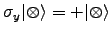 (so that
represents
a spin-
particle with its spin in the
(so that
represents
a spin-
particle with its spin in the  direction).
- TWO SPIN-
PARTICLES:
Suppose you have two spin-
particles,
such as a proton (
 ) and an electron (
 ),
whose magnetic moments
),
whose magnetic moments
 and
and
 interact with
an external magnetic field
interact with
an external magnetic field  , each contributing
its Zeeman energy
, each contributing
its Zeeman energy
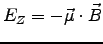 .
Then the Zeeman hamiltonian operator is
.
Then the Zeeman hamiltonian operator is
 |
(3) |
Again picking the
direction as the quantization axis,
we have four possible fully-specified quantum states:
![$\displaystyle \vert \! \Uparrow \uparrow \rangle
= \left[ {1 \atop 0} \atop {0 . . .
. . . \! \Downarrow \downarrow \rangle
= \left[ {0 \atop 0} \atop {0 \atop 1} \right]$](img33.gif) |
|
|
(4) |
where the
 and
and
 symbols designate
"spin up/down" (along the
axis) for the electron
and the proton, respectively.
symbols designate
"spin up/down" (along the
axis) for the electron
and the proton, respectively.
In this basis, verify that the  matrix representations
of the electron and proton spin operators are
matrix representations
of the electron and proton spin operators are
| |
![$\displaystyle \sigma_{e_2} = \left[\begin{matrix}
0 & 0 & -i & 0 \cr
0 & 0 & 0 & -i \cr
i & 0 & 0 & 0 \cr
0 & i & 0 & 0
\end{matrix}\right];$](img39.gif) |
![$\displaystyle \sigma_{p_2} = \left[\begin{matrix}
0 & -i & 0 & 0 \cr
i & 0 & 0 & 0 \cr
0 & 0 & 0 & -i \cr
0 & 0 & i & 0 \cr
\end{matrix}\right]$](img40.gif) |
(5) |
Given this information, write down the matrix representation of the
full Zeeman hamiltonian for these two spins in an arbitrary
magnetic field
 .
Express your result in terms of
.
Express your result in terms of  ,
,  and the
three components of
.
and the
three components of
.
- THE CONTACT INTERACTION:
Suppose your two spin-
particles
(e.g. the proton and the electron in a hydrogen atom)
interact in a way that depends only on the scalar
product of their spin vectors,6
 |
(6) |
where
 is the Heisenberg hamiltonian operator
and
is the Heisenberg hamiltonian operator
and  is the strength of the interaction, in energy units.
For simplicity, set
is the strength of the interaction, in energy units.
For simplicity, set  (i.e. measure all energies as multiples of
)
in this part.
(i.e. measure all energies as multiples of
)
in this part.
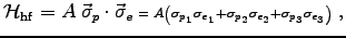
Express the Heisenberg spin hamiltonian (6)
as a matrix in the 4-state basis (4)
defined above,
and show that it is not diagonal.
Using MatLab, diagonalize it
and describe the new basis in which it is diagonal.7
- BREIT-RABI DIAGRAM: [EXTRA CREDIT]
We are now ready to solve the general problem of the
spin hamiltonian (which governs everything the spins do!)
of a hydrogen atom in an
 state with orbital
angular momentum
state with orbital
angular momentum  .8
The Breit-Rabi hamiltonian is
.8
The Breit-Rabi hamiltonian is
Express this hamiltonian in matrix form
for the 4-state basis (4)
and (using MatLab) diagonalize it
for some particular choice of applied magnetic field,
let's say
 .
Once you have accomplished this, you can repeat the
diagonalization for a succession of different values
of
.
Once you have accomplished this, you can repeat the
diagonalization for a succession of different values
of
 and plot the four energy eigenvalues
as a function of field to get the famous
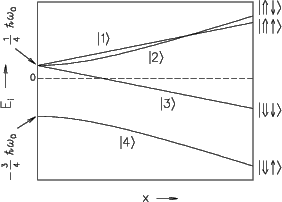
Breit-Rabi diagram for hydrogen:
and plot the four energy eigenvalues
as a function of field to get the famous
Breit-Rabi diagram for hydrogen:
Figure:
:
Breit-Rabi diagram showing the
energy levels of a system of two spin-1/2 particles
of opposite sign and different magnetic moments
(e.g. the hydrogen atom)
as functions of the reduced field
 where
where  (504.4 Oe for H in vacuum)
is a characteristic hyperfine field.
For the purpose of illustration, unphysical values
of moments and coupling constants have been used.
(504.4 Oe for H in vacuum)
is a characteristic hyperfine field.
For the purpose of illustration, unphysical values
of moments and coupling constants have been used.
 |
The actual hyperfine frequency
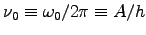 (where
  is Planck's constant)
has the value 1.42040575 GHz for hydrogen in vacuum.
In consistent units,
is Planck's constant)
has the value 1.42040575 GHz for hydrogen in vacuum.
In consistent units,
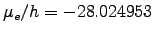 GHz/T
and
GHz/T
and
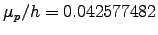 GHz/T.
In zero field the three triplet ( ) eigenstates
 ,
,  and
and  are degenerate
and the singlet (
are degenerate
and the singlet ( ) ground state
 is
is
 lower in energy.
At high reduced field (
 ) the eigenstates are
 ,
,
 ,
,
 and
and
 .
.
That is, the original basis!
Jess H. Brewer
2008-10-25
![$\displaystyle \sigma_{e_1} = \left[\begin{matrix}
0 & 0 & 1 & 0 \cr
0 & 0 & 0 & 1 \cr
1 & 0 & 0 & 0 \cr
0 & 1 & 0 & 0
\end{matrix}\right];$](img37.gif)
![$\displaystyle \sigma_{p_1} = \left[\begin{matrix}
0 & 1 & 0 & 0 \cr
1 & 0 & 0 & 0 \cr
0 & 0 & 0 & 1 \cr
0 & 0 & 1 & 0 \cr
\end{matrix}\right]$](img38.gif)
![$\displaystyle \sigma_{e_3} = \left[\begin{matrix}
1 & 0 & 0 & 0 \cr
0 & 1 & 0 & 0 \cr
0 & 0 & -1 & 0 \cr
0 & 0 & 0 & -1 \cr
\end{matrix}\right];$](img41.gif)
![$\displaystyle \sigma_{p_3} = \left[\begin{matrix}
1 & 0 & 0 & 0 \cr
0 & -1 & 0 & 0 \cr
0 & 0 & 1 & 0 \cr
0 & 0 & 0 & -1 \cr
\end{matrix}\right]$](img42.gif)