BELIEVE ME NOT! -  - A SKEPTIC's GUIDE


Next: Summary: The Exponential Function(s)
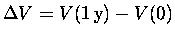
Suppose the newspaper headlines read,
"The cost of living went up 10% this year."
Can we translate this information into an equation?
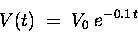
Let "V" denote the value of a dollar, in terms of
the "real goods" it can buy - whatever economists mean
by that. Let the elapsed time t be measured in years (y).
Then suppose that V is a function of t, V(t),
which function we would like to know explicitly.
Call now "t = 0" and let the initial value of the dollar
(now) be V0, which we could take to be $1.00 if we disregard
inflation at earlier times.1
Then our news item can be written
This formula can be rewritten in terms of the changes
in the dependent and independent variables,
 and
and
 :
:
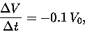 |
(1) |
where it is now to be understood that
V is measured in "1998 dollars"
and t is measured in years.
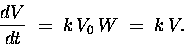
That is, the average time rate of change of V
is proportional to the value of V
at the beginning of the time interval,
and the constant of proportionality is -0.1 y-1.
(By y-1 or "inverse years" we mean the
per year rate of change.)
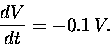
This is almost like a derivative.
If only  were infinitesimally small,
it would be a derivative.
Since we're just trying to describe the qualitative behaviour,
let's make an approximation: assume that
were infinitesimally small,
it would be a derivative.
Since we're just trying to describe the qualitative behaviour,
let's make an approximation: assume that
 year is "close enough"
to an infinitesimal time interval,
and that the above formula (1) for the inflation rate
can be turned into an instantaneous rate of change:2
year is "close enough"
to an infinitesimal time interval,
and that the above formula (1) for the inflation rate
can be turned into an instantaneous rate of change:2
 |
(2) |
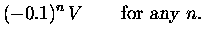
This means that the dollar in your pocket right now
will be worth only $0.99999996829 in one second.
Well, this is interesting, but we cannot go any further
with it until we ask a crucial question: "What will happen
if this goes on?" That is, suppose we assume that equation (2)
is not just a temporary situation, but
represents a consistent and ubiquitous property
of the function V(t), the "real value" of your dollar bill
as a function of time.3
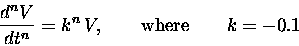
Applying the d/dt "operator" to both sides
of Eq. (2) gives
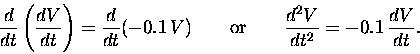 |
(3) |
But dV/dt is given by (2). If we substitute that formula
into the above equation (3), we get
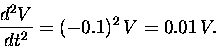 |
(4) |
That is, the rate of change of the rate of change is always
positive, or the (negative) rate of change is getting less
negative all the time.4
In general, whenever we have a positive second derivative
of a function (as is the case here), the curve is concave
upwards. Similarly, if the second derivative were negative,
the curve would be concave downwards.
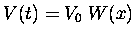
So by noting the initial value of V, which is formally
written V0 but in this case equals $1.00, and by applying
our understanding of the "graphical meaning"
of the first derivative (slope) and the second derivative
(curvature), we can visualize the function V(t) pretty well.
It starts out with a maximum downward slope
and then starts to level off as time increases.
This general trend continues indefinitely.
Note that while the function always decreases,
it never reaches zero.
This is because, the closer it gets to zero,
the slower it decreases [see Eq. (2)].
This is a very "cute" feature that makes this function
especially fun to imagine over long times.
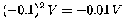
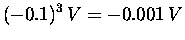
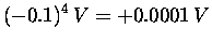
We can also apply our analytical understanding
to the formulas (2) and (4) for the derivatives:
every time we take still another derivative, the result
is still proportional to V - the constant of proportionality
just picks up another factor of (- 0.1). This is
a really neat feature of this function, namely
that we can write down all its derivatives
with almost no effort:
 |
= |
 |
(5) |
 |
= |
 |
(6) |
 |
= |
 |
(7) |
 |
= |
 |
(8) |
| |
 |
|
|
 |
= |
 |
(9) |
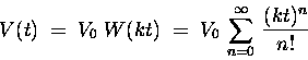
This is a pretty nifty function. What is it?
That is, can we write it down in terms of
familiar things like t, t2, t3, and so on?
First, note that Eq. (9) can be written in the form
 |
(10) |
A simpler version would be where k = 1, giving
 |
(11) |
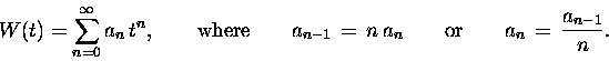
W(t) being the function satisfying this criterion.
We should perhaps try figuring out this simpler problem
first, and then come back to V(t).
Let's try expressing W(t), then, as a linear
combination5
of such terms.
For starters we will try a "third order polynomial"
(i.e. we allow terms up to t3):
follows by simple "differentiation" [a single word
for "taking the derivative"]. Now, these two equations
have similar-looking right-hand sides, provided that
we pretend not to notice that term in t3 in the first one,
and provided the constants an obey the rule
an-1 = n an [i.e. a0 = a1,
a1 = 2 a2 and
a2 = 3 a3].
But we can't really neglect that t3 term! To be sure,
its "coefficient" a3 is smaller than any of the rest,
so if we had to neglect anything it might be the best choice;
but we're trying to be precise, right? How precise?
Well, precise enough. In that case, would we be precise enough
if we added a term a4 t4, preserving the rule about
coefficients [
a3 = 4 a4]?
No? Then how about a5 t5?
And so on. No matter how precise an agreement with Eq. (11)
we demand, we can always take enough terms, using this
procedure, to achieve the desired precision. Even if
you demand infinite precision, we just [just?] take an
infinite number of terms:
 |
(12) |
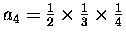
Now, suppose we give W(t) the initial value 1.
[If we want a different initial value
we can just multiply the whole
series by that value, without affecting Eq. (11).]
Well, W(0) = 1 tells us that a0 = 1.
In that case, a1 = 1 also, and
 ,
and
,
and
 ,
and
,
and
 ,
and so on. If we define the factorial notation,
,
and so on. If we define the factorial notation,
 |
(13) |
(read, "n factorial")
and define
 ,
we can express our function W(t)
very simply:
,
we can express our function W(t)
very simply:
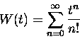 |
(14) |
We could also write a more abstract version of this function
in terms of a generalized variable "x":
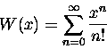 |
(15) |
Let's do this, and then define
 and set
 .
Then, by the CHAIN RULE for derivatives,6
.
Then, by the CHAIN RULE for derivatives,6
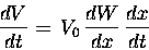 |
(16) |
and since
 ,
we have
,
we have
 |
(17) |
By repeating this we obtain Eq. (10). Thus
 |
(18) |
where k = - 0.1 in the present case.
This is a nice description; we can always calculate
the value of this function to any desired degree of accuracy
by including as many terms as we need until the change
produced by adding the next term is too small to worry us.7
But it is a little clumsy to keep writing down such an
unwieldy formula every time you want to refer to this
function, especially if it is going to be as popular as
we claim. After all, mathematics is the art of precise
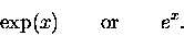
abbreviation. So we give W(x) [from Eq. (15)] a special name,
the "exponential" function, which we write as either8
 |
(19) |
In FORTRAN it is represented as EXP(X).
It is equal to the number
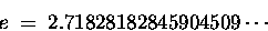 |
(20) |
raised to the
 power.
In our case we have
power.
In our case we have
 ,
so that our "answer" is
,
so that our "answer" is
 |
(21) |
which is a lot easier to write down than Eq. (18).
Now, the choice of notation ex is not arbitrary.
There are a lot of rules we know how to use on a number
raised to a power. One is that
 |
(22) |
You can easily determine that this rule also works
for the definition in Eq. (15).
The "inverse" of this function (the power to which
one must raise e to obtain a specified number)
is called the "natural logarithm" or " " function.
We write
" function.
We write
or
 |
(23) |
A handy application of this definition is the rule
![\begin{displaymath}y^x = e^{x \ln(y)} \qquad \hbox{\rm or} \qquad
y^x = \exp[x \ln(y)].
\end{displaymath}](img48.gif) |
(24) |
Before we return to our original function, is there
anything more interesting about the "natural logarithm"
than that it is the inverse of the "exponential" function?
And what is so all-fired special about e, the "base"
of the natural log? Well, it can easily be shown9
that the derivative of  is a very simple and familiar function:
![\begin{displaymath}{d[\ln(x)] \over dx} \; = \; {1 \over x} .
\end{displaymath}](img50.gif) |
(25) |
This is perhaps the most useful feature of ,
because
it gives us a direct connection between
the exponential function and
a function whose derivative is 1/x.
[The handy and versatile rule
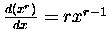 is valid for every value of r
but is no help with learning what function has the derivative 1/x.]
It also explains what is so special about the number e.
is valid for every value of r
but is no help with learning what function has the derivative 1/x.]
It also explains what is so special about the number e.
Next: Summary: The Exponential Function(s)
Jess H. Brewer -
Last modified: Fri Nov 13 17:21:02 PST 2015
![\begin{displaymath}\begin{array}[c]{ccrcrcrcl}
W(t) &=& a_0 &+& a_1 t &+& a_2 t...
...W \over dt}} &=& a_1 &+& 2 a_2 t &+& 3 a_3 t^2 & &
\end{array}\end{displaymath}](img23.gif)