BELIEVE ME NOT! -  - A SKEPTIC's GUIDE


Up: Calculus
Previous: Calculus
One thing that is easy to "read off a graph" of y(x) is the
slope of the curve at any given point x.
Now, if y(x) is quite "curved" at the point of interest,
it may seem contradictory to speak of its "slope,"
a property of a straight line.
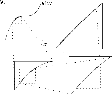
However, it is easy to see that as long as the curve is smooth
it will always look like a straight line
under sufficiently high magnification.
This is illustrated in Fig. 4.4 for a typical y(x)
by a process of successive magnifications.
Figure:
A series of "zooms" on a segment of the curve y(x)
showing how the curved line begins to look more and more
like a straight line under higher and higher magnification.
 |
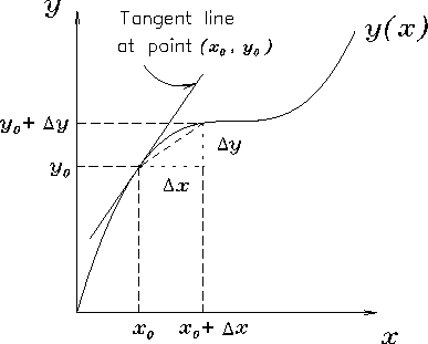
Figure:
A graph of the function y(x)
showing how the average slope
 is obtained on a finite interval of the curve.
By taking smaller and smaller intervals, one can eventually
obtain the slope at a point, dy/dx.
 |
We can also prescribe an algebraic method for calculating
the slope, as illustrated in Fig. 4.5:
the definition of the "slope" is the ratio of
the increase in y to the increase in x on a vanishingly
small interval. That is, when x goes from its initial value
x0 to a slightly larger value
 ,
the curve
carries y from its initial value
y0 = y(x0) to a new
value
 ,
and the slope
of the curve at x = x0 is given by
 for a vanishingly small
  .
When a small change like
 gets really small (i.e. small enough that
the curve looks like a straight line on that interval, or
"small enough to satisfy whatever criterion you want,"
then we write it differently, as dx, a "differential"
(vanishingly small) change in x.
Then the exact definition of the SLOPE of
y with respect to x at some particular value of x,
written in conventional Mathematical language, is
 |
(4.16) |
This is best understood by an example: consider the
simple function
y(x) = x2. Then
Divide this by  and we have
Now let  shrink to zero, and all that remains is
Thus the slope [or derivative,
as mathematicians are wont to call it] of
y(x) = x2
is
dy/dx = 2x. That is, the slope increases linearly
with x. The slope of the slope - which we call
the curvature, for obvious reasons - is then
trivially
 ,
a constant.
Make sure you can work this part out for yourself.
We have defined all these algebraic solutions to
the geometrical problem of finding the slope of a curve
on a graph in completely abstract terms - "x"
and "y" indeed! What are x and y?
Well, the whole idea is that they can be anything
you want! The most common examples in Physics
are when x is the elapsed time, usually
written t, and y is the distance travelled,
usually (alas) written x. Thus in an elementary
Physics context the function you are apt to see
used most often is x(t), the position of some object
as a function of time. This particular function has
some very well-known derivatives, namely
dx/dt = v, the speed or (as long as the motion
is in a straight line!) velocity of the object;
and
 ,
the acceleration
of the object. Note that both v and a are
themselves (in general) functions of time:
v(t) and a(t). This example so beautifully
illustrates the "meaning" of the slope and
curvature of a curve as first and second derivatives
that many introductory Calculus courses and virtually
all introductory Physics courses use it as the
example to explain these Mathematical conventions.
I just had to be different and start with something
a little more formal, because I think you will find that
the idea of one thing being a function of
another thing, and the associated ideas of graphs
and slopes and curvatures, are handy notions worth
putting to work far from their traditional realm of
classical kinematics.


Up: Calculus
Previous: Calculus
Jess H. Brewer -
Last modified: Fri Nov 13 16:21:19 PST 2015
 - A SKEPTIC's GUIDE
  - A SKEPTIC's GUIDE

![]() ,
the curve
carries y from its initial value
y0 = y(x0) to a new
value
,
the curve
carries y from its initial value
y0 = y(x0) to a new
value
![]() ,
and the slope
of the curve at x = x0 is given by
,
and the slope
of the curve at x = x0 is given by
![]() for a vanishingly small
for a vanishingly small ![]() .
When a small change like
.
When a small change like
![]() gets really small (i.e. small enough that
the curve looks like a straight line on that interval, or
"small enough to satisfy whatever criterion you want,"
then we write it differently, as dx, a "differential"
(vanishingly small) change in x.
Then the exact definition of the SLOPE of
y with respect to x at some particular value of x,
written in conventional Mathematical language, is
gets really small (i.e. small enough that
the curve looks like a straight line on that interval, or
"small enough to satisfy whatever criterion you want,"
then we write it differently, as dx, a "differential"
(vanishingly small) change in x.
Then the exact definition of the SLOPE of
y with respect to x at some particular value of x,
written in conventional Mathematical language, is